NumPy Concatenate, Stack, Split, and Append

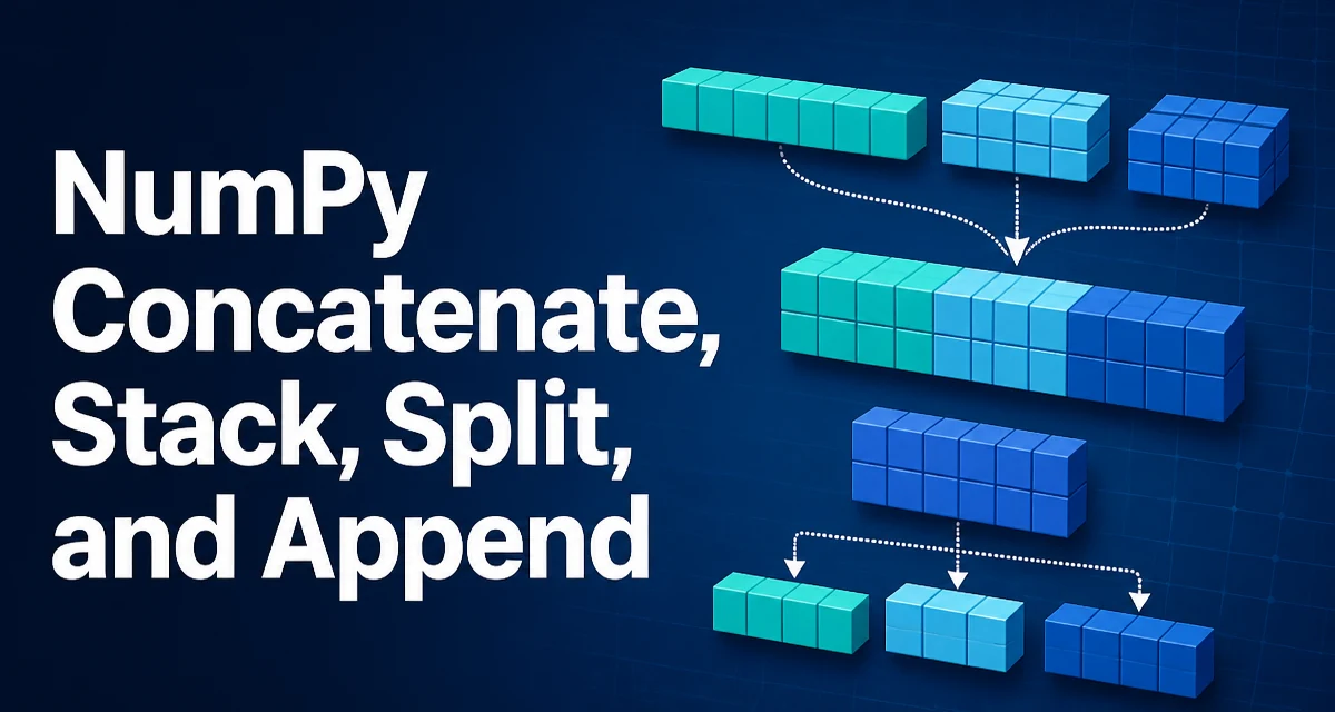
python numpy concatenate stack split and append requires a clear understanding of the core syntax, runtime behavior, and practical implementation patterns demonstrated in the examples below.

When working with NumPy arrays, combining and dividing them is a constant task. The functions concatenate, stack, split, and append are the primary tools for this, but they behave differently in ways that affect the shape of your data and the performance of your code. Choosing the wrong one often produces an unexpected shape or an unnecessary copy of your data. This article explains what each function does, how they differ, and when to use each.

The Difference Between Concatenate and Stack

np.concatenate joins a sequence of arrays along an existing axis. If you have two 1D arrays and concatenate them, you get a longer 1D array. If you concatenate two 2D arrays along axis 0, you add rows; along axis 1, you add columns. The key constraint is that the arrays must have the same shape along every axis except the one you are joining on.

np.stack is different. It creates a new axis and places each input array along that axis. Given two arrays of shape (3,), np.stack with default axis=0 produces an array of shape (2, 3). The input arrays are not required to match in the same way because they are simply placed into a new dimension.

import numpy as np

a = np.array([1, 2, 3])
b = np.array([4, 5, 6])

print(np.concatenate([a, b]))  # [1 2 3 4 5 6]
print(np.stack([a, b]))        # [[1 2 3]
                               #  [4 5 6]]

This distinction matters because concatenate preserves the number of dimensions, while stack adds one. If you need a matrix where each row is an original array, stack is the direct choice. If you need a flat sequence, concatenate is correct.

Using the axis Parameter Correctly

The axis parameter controls which dimension is joined. For concatenate, axis=0 joins along rows, axis=1 along columns, and higher values work for higher-dimensional arrays. A common mistake is forgetting that axis=0 is the default, which is fine for 1D arrays but may not be what you want for 2D data.

x = np.array([[1, 2], [3, 4]])
y = np.array([[5, 6]])

# Add a row
row_combined = np.concatenate([x, y], axis=0)
# array([[1, 2],
#        [3, 4],
#        [5, 6]])

# Add a column (requires matching row counts)
z = np.array([[7], [8]])
col_combined = np.concatenate([x, z], axis=1)
# array([[1, 2, 7],
#        [3, 4, 8]])

When using stack, the axis parameter refers to the position of the new axis in the output. For two arrays of shape (2, 2), np.stack([x, y], axis=0) produces shape (2, 2, 2), while axis=2 also produces (2, 2, 2) but with the new axis last. This distinction is subtle but critical when you need to match a specific data layout for machine learning or scientific computation.

Splitting Arrays with split and its Variants

np.split divides an array into multiple sub-arrays. You can specify either the number of equal parts or the exact indices where the split should occur. If the array cannot be divided evenly and you request equal parts, NumPy raises a ValueError. The array_split function is more forgiving: it allows unequal divisions without raising an error.

data = np.arange(10)

parts = np.split(data, 5)
# [array([0, 1]), array([2, 3]), array([4, 5]), array([6, 7]), array([8, 9])]

parts = np.array_split(data, 3)
# [array([0, 1, 2, 3]), array([4, 5, 6]), array([7, 8, 9])]

For 2D arrays, np.split works along a specified axis. You can split along rows or columns by passing the appropriate axis value. This is useful when partitioning a dataset into training and validation sets, or when processing blocks of a matrix independently.

matrix = np.arange(12).reshape(3, 4)
rows = np.split(matrix, 3, axis=0)
# Each element has shape (1, 4)

There are also hsplit and vsplit for horizontal and vertical splits, which are convenient wrappers that avoid specifying the axis explicitly. hsplit splits along columns, and vsplit splits along rows.

Append: A Convenience Function with a Catch

np.append is a convenience wrapper around concatenate. It flattens the input arrays before concatenation unless the axis parameter is provided. This is the most common source of confusion. If you call np.append(a, b) on two 2D arrays without specifying axis, the result is a 1D array, not a 2D array.

a = np.array([[1, 2], [3, 4]])
b = np.array([[5, 6]])

flat = np.append(a, b)  # array([1, 2, 3, 4, 5, 6])
with_axis = np.append(a, b, axis=0)  # array([[1, 2], [3, 4], [5, 6]])

Because np.append returns a new array and copies the data, using it repeatedly in a loop is inefficient. Each call allocates a new array and copies the existing data plus the new element, leading to O(n²) behavior. For incremental growth, a Python list with a final conversion to a NumPy array is usually faster and clearer.

Memory and Performance Considerations

All of these functions return new arrays; they do not modify the input in place. This means that combining large arrays creates a full copy of the data. If you are working with arrays that are hundreds of megabytes or larger, repeated concatenation or append operations can cause significant memory pressure and slow down your program.

A common pattern is to collect pieces in a list and call np.concatenate once at the end. This avoids the repeated copying of incremental append calls.

pieces = []
for i in range(1000):
    pieces.append(np.array([i, i * 2]))

result = np.concatenate(pieces)

This approach allocates the final array once and copies each piece into it, rather than reallocating and copying the entire result after each addition. For most batch-processing scenarios, this is the recommended pattern.

Choosing the Right Function for the Task

Use concatenate when you are joining arrays that already share the correct dimensionality. Use stack when you need to add a new axis, such as creating a batch dimension for model input. Use split or array_split when partitioning data, and use append only for simple cases where the flattening behavior is acceptable or where you explicitly pass axis.

Handling Edge Cases and Common Errors

A frequent error is passing arrays with incompatible shapes to concatenate. For example, concatenating a (2, 3) array with a (2, 4) array along axis 0 fails because the second dimension does not match. The error message states that all input array dimensions except for the concatenation axis must match exactly.

Another edge case is splitting an array into more parts than it has elements. np.split raises a ValueError in this situation. np.array_split can handle it, but it will produce some empty arrays. If empty arrays are not acceptable, you need to check the length before splitting.

For stack, the input arrays must have the same shape. Unlike concatenate, there is no exception for a join axis, because every dimension is preserved and a new one is added. This makes stack stricter in one sense but more flexible in another: it does not require the arrays to be compatible along any existing dimension.

Practical Example: Building a Feature Matrix

Suppose you have a list of sensor readings, each being a 1D array of measurements. You want to build a 2D matrix where each row corresponds to one sensor. This is a natural fit for np.stack.

readings = [
    np.array([1.2, 2.3, 3.4]),
    np.array([4.5, 5.6, 6.7]),
    np.array([7.8, 8.9, 9.0]),
]

feature_matrix = np.stack(readings, axis=0)
print(feature_matrix.shape)  # (3, 3)

If instead you had a stream of new readings arriving one at a time and you wanted to add them to the matrix, you would use np.concatenate with axis=0, but only if you are certain the new reading has the same length as the existing rows.

new_reading = np.array([1.0, 2.0, 3.0])
feature_matrix = np.concatenate([feature_matrix, new_reading[None, :]], axis=0)

The new_reading[None, :] adds a new axis so the array has shape (1, 3), making it compatible with concatenate along axis 0. This is a common idiom that avoids accidentally flattening the data.

Compatibility and Version Considerations

The behavior of these functions has been stable across recent NumPy versions, but there are a few points worth noting. np.append has always flattened input without an axis, and this is unlikely to change because it would break existing code. The axis parameter for np.stack was introduced in NumPy 1.10, so very old codebases may not have access to it. For most modern environments, this is not a concern, but if you maintain code that runs on legacy systems, verify the NumPy version before relying on newer features.

Also, these functions work on any array-like input, not just ndarray objects. Passing Python lists or tuples will cause NumPy to convert them internally. However, the return type is always an ndarray. If you need to preserve a specific subclass or a masked array, you may need to use the corresponding methods on that class rather than the top-level functions. For example, masked arrays have their own concatenate and stack methods that preserve the mask metadata. Using the generic functions on masked arrays can drop the mask, which is a subtle but important data loss. In such cases, prefer the class-specific methods or verify the mask is retained after the operation.