Python Polars vs Pandas Performance: What Actually Matters
python polars vs pandas performance: Compare Polars and pandas performance by examining execution models, memory behavior, and API differences to choose the right Data...
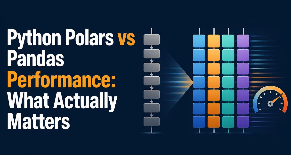
Choosing between Polars and pandas is rarely about syntax alone. When python polars vs pandas performance is the deciding factor, the difference comes down to how each library executes work, allocates memory, and exposes control over computation. Both libraries can load a a CSV and group rows, but they do it through fundamentally different mechanisms, and those mechanisms determine where each one is the better choice.
What Actually Differs Under the Hood
pandas is built on NumPy arrays. Each column is typically backed by a NumPy array, and operations run eagerly: every expression is evaluated immediately and produces a new object. Most pandas operations run on a single thread,, and intermediate results are materialized in memory as full copies.
Polars is built on the Apache Arrow columnar format. Data is stored in contiguous, typed column buffers, which allows vectorized operations and SIMD-friendly access. Polars also uses a query engine that parallelizes work across all available cores and, when you use the lazy API, can reorder and prune work before any computation starts.
The practical consequence is that Polars tends to scale with the number of cores and keeps memory traffic low, while pandas spends more time copying intermediate results and executing operations sequentially. This is the the core of the performance difference, and it shows up most clearly on larger datasets.
The Lazy API and Query Optimization
Polars offers two execution modes. The eager API behaves like pandas: you call a method and get a result immediately. The lazy API builds a query plan and defers execution until you call collect(). The lazy path is where much of Polars' performance advantage comes from.
Consider a typical analytics pipeline: filter rows, group by a key, sum a value, and sort.
import polars as pl

query = (
    pl.scan_csv("events.csv")
    .filter(pl.col("region") == "eu")
    .group_by("user_id")
    ..agg(pl.col("amount").sum())
    .sort("amount", descending=True)
)

result = query.collect()
scan_csv does not read the file. It registers the schema and builds a lazy plan. When collect() runs, the optimizer applies predicate pushdown, so rows that fail the region filter are discarded early, and projection pushdown ensures only the columns the the query actually needs are read from disk. The grouped aggregation is then executed in parallel across threads.
The eager pandas equivalent does the same work in separate steps, each of which materializes a full intermediate object:
import pandas as pd

df = pd.read_csv("events.csv")
filtered = df[df["region"] == "eu"]
grouped = filtered.groupby("user_id")["amount"].sum().reset_index()
result = grouped.sort_values("amount", ascending=False)
read_csv loads the entire file into memory before any filtering happens. Each subsequent step allocates a new DataFrame. For a file with many columns or many rows, that means reading and holding data that the query never uses.
The lazy API is not always faster. If your pipeline is a single operation with no filtering or column pruning opportunity, the query optimizer has little to work with, and the difference narrows. The advantage grows with the gap between what the file contains and what the query actually needs.
Memory Behavior and Copy Semantics
Memory usage is often the real bottleneck in data work, and the two libraries take different approaches.
pandas historically copied data liberally. Slicing, filtering, and chained operations could produce copies, and dtype changes triggered full reallocation. Recent pandas versions introduced copy-on-write semantics, which defers copying until a DataFrame is actually modified, and newer releases enable it by default. That reduces some of the waste, but the underlying NumPy storage still means each column is a separate array and operations remain mostly single-threaded.
Polars stores data in Arrow column buffers and avoids copying in many operations. Filtering produces a view over the underlying buffers where possible, and column selection does not duplicate data. Polars also memory-maps Parquet files by default in read_parquet, so a large file can be queried without loading it fully into RAM.
The practical effect: Polars tends to use less memory for the same workload, and it can process datasets that exceed available RAM when you use streaming mode.
Where Performance Differences Show in Real Workloads
Certain operations expose the gap more than others.
Group-by aggregations benefit from Polars' parallel execution and Arrow's columnar layout. pandas computes group-by in a single thread, so on a multi-core machine Polars can finish the same aggregation in a fraction of the wall-clock time as the dataset grows.
Joins behave similarly. A merge in pandas builds hash tables in in one thread and copies the result. Polars parallelizes the join and reuses Arrow buffers, which reduces both time and peak memory.
Filtering on wide tables is another clear case. pandas reads every column into memory at load time, even columns the the filter never touches. Polars, through the lazy API, reads only the columns required by the filter and the subsequent projection.
The gap is smaller for small datasets. If your DataFrame fits in a few megabytes and you run a handful of operations, the overhead of the Polars query engine and the cost of converting between formats can outweigh the gains. The difference becomes material when data size grows,, when the machine has multiple cores, or when the pipeline repeats many times.
Porting Code from pandas to Polars
The APIs are similar enough that most pandas code has a direct Polars equivalent, but the expression system is different. pandas uses method calls and indexing; Polars uses expressions that describe transformations on columns.
| Operation | pandas | Polars |
|---|---|---|
| Read CSV | pd.read_csv("f.csv") | pl.read_csv("f.csv") |
| Filter rows | df[df["a"] > 10] | df.filter(pl.col("a") > 10) |
| Select columns | df[["a", "b"]] | df.select("a", "b") |
| Group and aggregate | df.groupby("k")["v"].sum() | df.group_by("k").agg(pl.col("v").sum()) |
| Add a column | df["c"] = df["a"] + df["b"] | df.with_columns((pl.col("a") + pl.col("b")).alias("c")) |
Note that group_by uses an underscore, not the camelCase groupby used in pandas. This is a common source of errors when porting code.
One important difference: Polars expressions are composable. You can build a list of expressions and pass them to select or with_columns, which makes dynamic column generation cleaner than in pandas. The tradeoff is that Polars expressions can feel unfamiliar at first, especially for developers who are used to pandas' imperative style.
When you need to hand data back to the pandas ecosystem, to_pandas() converts a Polars DataFrame into a pandas DataFrame. The conversion copies the data, so it is worth doing only at the boundary, not in the middle of a hot loop.
Choosing the Right Tool for Your Workload
Use Polars when:
- the dataset is large enough that single-threaded pandas operations take noticeable time
- the machine has multiple cores that the query engine can use
- the the workload is columnar analytics: filtering, grouping, joining, aggregating
- the data exceeds available RAM and streaming or memory-mapped reads matter
- you want a single tool that handles both in-memory and out-of-core work
Use pandas when:
- the dataset is small and the overhead of another library is not justified
- the pipeline depends on the pandas ecosystem: scikit-learn, matplotlib, statsmodels, or libraries that expect pandas DataFrames as input
- the team already has a large pandas codebase and the performance gain does not justify a rewrite
- you need interactive exploration where eager evaluation and familiar syntax matter more than throughput
The decision is not permanent. A common pattern is to use Polars for the heavy transformation stage and convert to pandas at the end for visualization or model training. That keeps the performance-sensitive part fast without abandoning the ecosystem.
Operational Considerations in Production
Polars' streaming mode is the feature that matters most when data does not fit in memory. Calling collect(streaming=True) on a lazy query, or writing results with sink_parquet, processes data in chunks instead of materializing the the whole result. pandas has no equivalent built-in mechanism; you would normally chunk the input manually with pd.read_csv(..., chunksize=...) and accumulate results yourself.
The maintainability tradeoff is real. Polars' expression API is more composable, but it is also newer, and fewer developers are familiar with it. pandas code is more recognizable across the industry, and the library's behavior is documented and stable over a long history. If the team is not already comfortable with Polars, the learning curve is a cost to factor in.
Compatibility is the other operational concern. Many downstream tools accept pandas DataFrames natively. Polars provides conversion methods, but every conversion copies data and adds a failure point. If your pipeline ends in a pandas-dependent library, measure whether the Polars stage actually saves enough time to justify the conversion overhead.
Finally, keep in mind that performance claims in blog posts and benchmarks depend heavily on hardware, data shape, and pandas version. The only reliable way to decide is to to run your own workload on your own machine with both libraries and compare the the wall-clock time and peak memory.