Python PyTorch nn Module Layers and Activation Functions
python pytorch nn module layers and activation functions: Learn how to use torch.nn layers and activation functions to build neural networks in PyTorch, with practical...
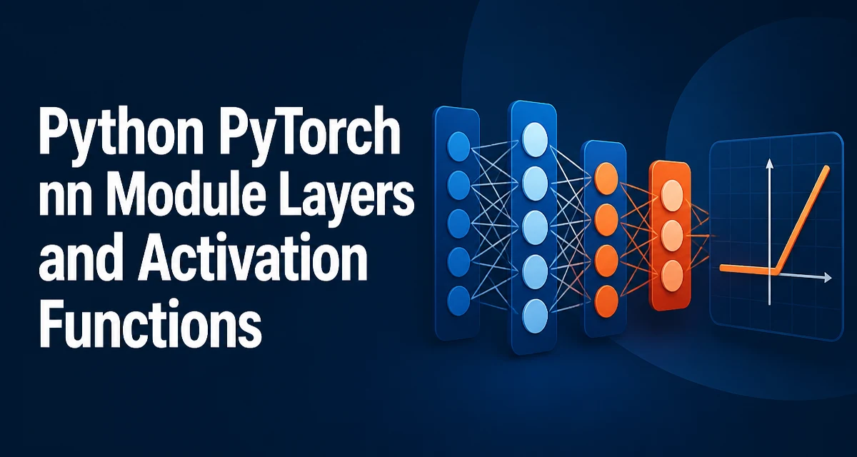
python pytorch nn module layers and activation functions requires a clear understanding of the core syntax, runtime behavior, and practical implementation patterns demonstrated in the examples below.
When working with PyTorch, the torch.nn module provides the building blocks for constructing neural networks. Understanding how to use nn.Module layers and activation functions is essential for implementing models in Python. This article covers the core components, how to combine them into a working model, and the tradeoffs you should consider when choosing layers and activations.
Core Layers in torch.nn
The torch.nn module includes a wide range of layer types, each designed for a specific kind of transformation. The most commonly used layers are nn.Linear, nn.Conv2d, nn.LSTM, and nn.Embedding. Each layer is a subclass of nn.Module and implements a forward method that defines the transformation applied to its input.
For a fully connected network, nn.Linear is the fundamental building block. It applies an affine transformation: y = xW^T + b. Here is a minimal example:
import torch
import torch.nn as nn

linear = nn.Linear(in_features=16, out_features=8)
x = torch.randn(4, 16)
y = linear(x)
print(y.shape)  # torch.Size([4, 8])
The in_features and out_features arguments determine the shape of the weight matrix. The weight and bias are automatically initialized, but you can override them later if needed.
For image data, nn.Conv2d is the standard choice. It applies a 2D convolution over an input of shape (N, C_in, H, W). The key parameters are in_channels, out_channels, kernel_size, stride, and padding. For example:
conv = nn.Conv2d(in_channels=3, out_channels=16, kernel_size=3, padding=1)
x = torch.randn(1, 3, 32, 32)
y = conv(x)
print(y.shape)  # torch.Size([1, 16, 32, 32])
Padding is crucial to control the spatial dimensions of the output. Without padding, a 3x3 kernel reduces a 32x32 input to 30x30. The same principle applies to other convolution variants like nn.Conv1d and nn.Conv3d.
Activation Functions as nn.Module
Activation functions introduce non-linearity into the network, allowing it to learn complex patterns. PyTorch provides these as both nn.Module subclasses and functional versions in torch.nn.functional. The module versions are typically used when building models with nn.Sequential or when you need to store them as attributes.
Common activation functions include nn.ReLU, nn.Sigmoid, nn.Tanh, and nn.LeakyReLU. Each has a distinct mathematical form and practical implications. For instance, nn.ReLU is defined as max(0, x) and is the default choice for hidden layers in many architectures because it mitigates the vanishing gradient problem.
relu = nn.ReLU()
x = torch.tensor([-1.0, 0.0, 2.0])
print(relu(x))  # tensor([0., 0., 2.])
nn.Sigmoid squashes values to the range (0, 1) and is often used in the output layer for binary classification. However, it suffers from saturation, which can slow down training. nn.Tanh outputs values between -1 and 1 and is sometimes used in recurrent networks.
When you need a specific slope for negative inputs, nn.LeakyReLU is a practical alternative. It allows a small gradient when the input is negative, which can prevent dead neurons.
Building a Custom Model with nn.Module
The standard way to define a neural network in PyTorch is to subclass nn.Module. You declare layers as attributes in __init__ and define the forward pass in the forward method. This gives you full control over how data flows through the network.
class SimpleMLP(nn.Module):
    def __init__(self, input_size, hidden_size, output_size):
        super().__init__()
        self.fc1 = nn.Linear(input_size, hidden_size)
        self.relu = nn.ReLU()
        self.fc2 = nn.Linear(hidden_size, output_size)

    def forward(self, x):
        x = self.fc1(x)
        x = self.relu(x)
        x = self.fc2(x)
        return x
The forward method is called when you invoke the model on an input. PyTorch automatically tracks operations for gradient computation, so you do not need to manually implement backpropagation. The model's parameters are accessible via model.parameters() and can be passed to an optimizer.
Using nn.Sequential for Simple Architectures
For straightforward feed-forward networks, nn.Sequential is a convenient container that chains layers in order. It reduces boilerplate and makes the architecture explicit.
model = nn.Sequential(
    nn.Linear(784, 256),
    nn.ReLU(),
    nn.Linear(256, 10)
)
nn.Sequential is ideal when the forward pass is a simple sequence of operations. However, it does not allow branching or skip connections. For more complex flows, you need a custom nn.Module subclass.
One subtlety is that nn.Sequential stores layers as submodules, so they appear in model.parameters() and can be moved to a GPU with model.cuda().
Parameter Management and Initialization
Every layer has parameters that are automatically initialized using default schemes. For nn.Linear, the weight is initialized using Kaiming uniform initialization, and the bias is set to a small constant. You can override these defaults by accessing the layer's weight and bias attributes.
def init_weights(m):
    if isinstance(m, nn.Linear):
        nn.init.xavier_uniform_(m.weight)
        nn.init.zeros_(m.bias)

model.apply(init_weights)
Applying a custom initialization is common when you need a specific distribution or when you are working with pre-trained models. The apply method recursively applies a function to every submodule, which is useful for uniform initialization across all layers.
Parameter management also involves freezing layers during fine-tuning. You can set param.requires_grad = False to prevent updates. This is often done for the earlier layers of a pre-trained network.
Functional API vs Module API
PyTorch offers activation functions and some layers in both torch.nn.functional and as nn.Module subclasses. For example, F.relu and nn.ReLU perform the same operation, but they differ in how they are used.
The functional version is stateless and is typically called inside a custom forward method. It does not hold any parameters or buffers, which makes it lighter. The module version, on the other hand, can be used as part of nn.Sequential and may have additional attributes (like inplace for ReLU).
import torch.nn.functional as F

def forward(self, x):
    x = F.relu(self.fc1(x))
    return x
Using the functional API is a common pattern in research code because it avoids storing unnecessary module instances. However, if you need to track the activation as a submodule (e.g., for visualization), the module version is more convenient.
Performance and Memory Considerations
When building models, the choice between inplace operations and standard operations can affect memory usage. For example, nn.ReLU(inplace=True) modifies the input tensor directly, potentially saving memory because it does not create a new tensor. However, inplace operations can interfere with gradient computation if the input is needed for the backward pass. PyTorch handles this by copying the input when necessary, but it can still lead to subtle bugs if you reuse the same tensor elsewhere.
Another performance factor is the placement of activation functions. Applying a non-linearity immediately after a linear layer is standard, but you should avoid redundant activations. For instance, using ReLU twice in a row is equivalent to a single ReLU and wastes computation.
For large models, moving data to the GPU and using batch processing is essential. Layers like nn.Linear and nn.Conv2d are optimized for GPU execution, but the overhead of transferring data between CPU and GPU can dominate if the batch size is too small.
Choosing Layers and Activation Functions for Your Task
The right layer and activation depend on the problem domain. For tabular data, nn.Linear layers with ReLU activations are a solid baseline. For image classification, convolutional layers followed by ReLU and pooling are standard. For sequence data, recurrent layers like nn.LSTM or transformer layers are more appropriate.
Activation selection also matters. ReLU is fast and works well for most hidden layers, but it can suffer from dead neurons when the learning rate is too high. LeakyReLU or ELU can mitigate this. For the output layer, Softmax is used for multi-class classification, Sigmoid for binary classification, and no activation for regression tasks.
A practical approach is to start with ReLU for hidden layers and Softmax for classification, then experiment with alternatives if training stalls. The choice is not arbitrary; it affects gradient flow and convergence speed. For example, Tanh is often preferred in recurrent networks because its outputs are centered around zero, which can improve numerical stability.
When you need to combine layers and activations, nn.Sequential provides a concise way to define the architecture. For more complex models, subclassing nn.Module gives you the flexibility to implement custom forward logic, such as residual connections or multi-branch designs. Understanding the tradeoffs between these approaches helps you write models that are both correct and efficient.