Python SciPy Integrate Interpolation and Numerical Methods

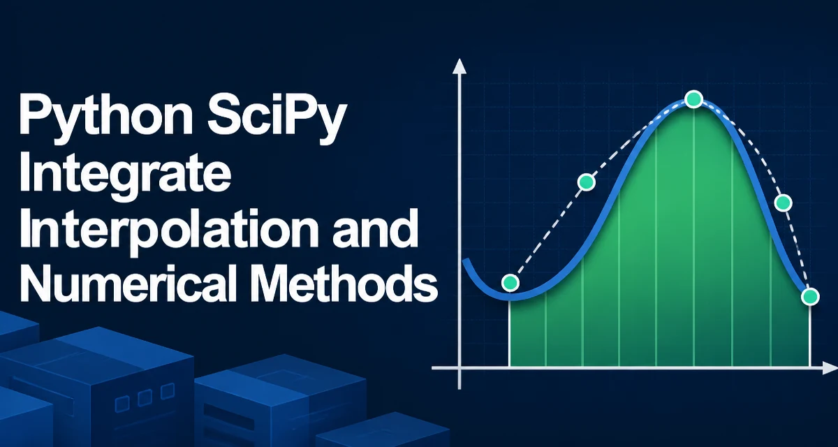
When you need to apply python scipy integrate interpolation and numerical methods to real data, SciPy provides a consistent set of routines that handle the heavy lifting. The library separates concerns into submodules: scipy.integrate for quadrature and ODE solving, scipy.interpolate for constructing functions from discrete data, and scipy.optimize for root finding and minimization. This article focuses on the integration and interpolation pieces, plus the ODE solvers that often accompany them.

The SciPy Toolset for Integration, Interpolation, and ODEs

SciPy's numerical stack is built on NumPy arrays and provides low-level routines that are both fast and well tested. For most scientific computing tasks, you do not need to implement Simpson's rule or a cubic spline from scratch. Instead, you call a function that has been validated against known test cases and tuned for accuracy and performance.

The three submodules you will use most often are:

• scipy.integrate – for definite integrals and initial value problems.
• scipy.interpolate – for building continuous functions from discrete samples.
• scipy.optimize – for finding roots, minima, and curve fitting, which often complements the other two.

This article assumes you have SciPy installed and are comfortable with NumPy arrays. The examples use Python 3 and SciPy 1.x, but the core APIs have been stable for many releases.

Numerical Integration with scipy.integrate

The most common integration task is computing a definite integral of a known function. The quad function from scipy.integrate handles this with an adaptive Gauss-Kronrod method. It returns both the integral value and an estimate of the absolute error.

from scipy.integrate import quad

def f(x):
    return x**2

result, error = quad(f, 0, 1)
print(result)  # 0.3333333333333333
print(error)   # 3.700743415417189e-15

quad accepts a callable and the integration limits. It can also handle infinite limits, singularities, and parameters passed through the args argument. For example, to integrate a function with a parameter:

def g(x, a):
    return a * x**2

result, error = quad(g, 0, 1, args=(3,))

When you have tabulated data instead of a function, use simpson (formerly simps) or trapezoid. These functions take arrays of x and y values and approximate the integral using the corresponding rule.

import numpy as np
from scipy.integrate import simpson

x = np.linspace(0, 1, 100)
y = x**2
area = simpson(y, x)

The simpson function works with sampled points that are not necessarily evenly spaced, which is common in experimental data. For evenly spaced points, trapezoid is simpler but less accurate for smooth functions.

Interpolation with scipy.interpolate

Interpolation constructs a function that passes exactly through the given data points. The simplest class is interp1d, which creates a 1-D interpolation function that can be evaluated at any point within the original range.

from scipy.interpolate import interp1d

x = np.array([0, 1, 2, 3, 4])
y = np.array([0, 1, 4, 9, 16])
f_interp = interp1d(x, y, kind='quadratic')

x_new = 2.5
y_new = f_interp(x_new)

The kind parameter controls the interpolation order: 'linear', 'quadratic', 'cubic', or a spline order. For smooth data, 'cubic' often gives the best visual result, but it can overshoot if the data has sharp changes.

For more control, use UnivariateSpline from the same module. It allows you to specify a smoothing factor, which trades off between fitting the data exactly and producing a smoother curve. This is useful when your data contains noise.

from scipy.interpolate import UnivariateSpline

spline = UnivariateSpline(x, y, s=0.5)
y_smooth = spline(x_new)

When your data is scattered in 2-D or higher, griddata and RBFInterpolator are the tools to use. griddata interpolates unstructured data onto a grid, which is common in visualization and contour plotting.

Solving Ordinary Differential Equations

Many physical systems are described by ODEs. SciPy's solve_ivp is the modern interface for initial value problems. It replaces the older odeint and offers more control over the integration method.

from scipy.integrate import solve_ivp

def dydt(t, y):
    return -2 * y

sol = solve_ivp(dydt, [0, 5], [1], method='RK45')

The first argument is the derivative function, which takes time t and state vector y. The second is the time span, and the third is the initial condition. The method parameter selects the solver: 'RK45' for non-stiff problems, 'Radau' or 'BDF' for stiff problems.

solve_ivp returns an object with attributes t and y, which contain the time points and the solution values. You can also evaluate the solution at specific times using the t_eval argument.

sol = solve_ivp(dydt, [0, 5], [1], t_eval=np.linspace(0, 5, 100))

For systems of equations, y is a vector and the derivative function returns an array of the same shape. This is a common pattern in physics and engineering simulations.

Choosing the Right Method for Your Data

The choice between integration, interpolation, and ODE solving is usually dictated by the problem structure, but within each category you still need to pick the right algorithm.

For integration, use quad when you have a continuous function and need high accuracy. Use simpson or trapezoid when you only have sampled data. If the data is noisy, consider smoothing it before integration, but be aware that smoothing introduces bias.

For interpolation, the decision is between interp1d and UnivariateSpline. interp1d is simpler and always passes through the data points. UnivariateSpline allows smoothing and gives you a spline object that can be differentiated and integrated. If your data is noisy, UnivariateSpline with a positive smoothing factor is often the better choice.

For ODEs, the main decision is whether the problem is stiff. Non-stiff problems are efficiently solved with RK45. Stiff problems require implicit methods like Radau or BDF. You can detect stiffness by trying RK45 and observing if it takes very small steps or fails to converge.

Performance and Numerical Accuracy Considerations

SciPy routines are implemented in compiled Fortran and C, so they are fast for moderate-sized problems. The main performance bottleneck is usually the number of function evaluations. For integration, the adaptive algorithm evaluates the function many times, so make sure your function is vectorized when possible.

For interpolation, building a spline is an O(n) operation, but evaluating it is O(1) for interp1d with linear or cubic splines. If you need to evaluate the interpolant many times, reuse the same object instead of recreating it.

For ODE solvers, the step size is controlled by the error tolerance. Setting rtol and atol to appropriate values can reduce computation time without sacrificing accuracy. A common starting point is rtol=1e-6 and atol=1e-9, but you should adjust based on the scale of your variables.

Common Pitfalls and How to Avoid Them

One frequent mistake is using interpolation to extrapolate beyond the data range. Most interpolation methods in SciPy raise an error or produce meaningless values outside the original domain. Always check the bounds of your data before evaluating an interpolant.

Another issue is mixing up the order of arguments in interp1d. The first argument is the independent variable, and the second is the dependent variable. Swapping them leads to a silently wrong result.

When solving ODEs, remember that solve_ivp expects the derivative function to accept t first and y second. This is the opposite of the older odeint signature, which takes y first. If you are migrating code, check the argument order.

Finally, be careful with the method parameter in solve_ivp. Using 'RK45' on a stiff problem can produce inaccurate results or take an extremely long time. If you suspect stiffness, switch to 'BDF' or 'Radau' and compare the solutions.