Python SciPy Signal Processing and FFT: Core Workflows

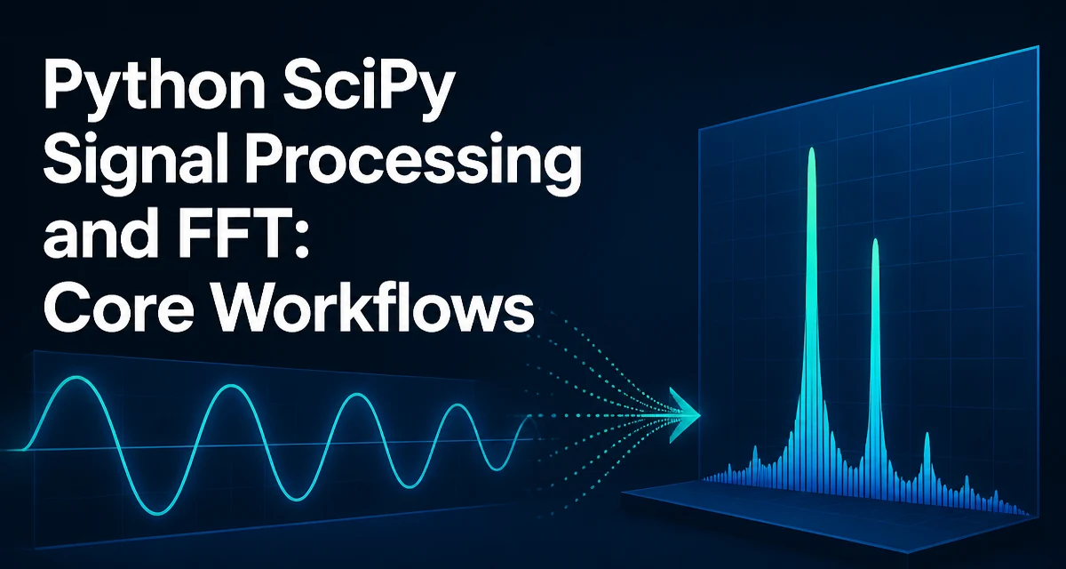
Python's SciPy library provides a complete toolkit for signal processing, and its FFT implementation is the foundation of most frequency-domain work. The scipy.fft module offers fast, well-tested transforms that integrate cleanly with NumPy arrays, while scipy.signal supplies filtering and windowing utilities that complete a typical analysis pipeline. This article covers the practical workflow for python scipy signal processing and fft: computing a spectrum, interpreting the output, filtering in the frequency domain, and reconstructing a signal.

The scipy.fft Module and Its Core Functions

The scipy.fft module, available since SciPy 1.4, provides the core transforms you will use for most frequency-domain analysis. The main functions are:

• fft and ifft — general-purpose forward and inverse transforms
• rfft and irfft — optimized variants for real-valued input
• fftfreq and rfftfreq — generate the frequency bin centers for a given transform length and sample spacing

Unlike numpy.fft, scipy.fft uses the pocketfft backend, which handles a wider range of input lengths efficiently and supports worker threads for parallel execution. The API is nearly identical to numpy.fft, so code can switch between the two with minimal changes. For new signal-processing work, prefer scipy.fft because it integrates with the rest of the SciPy ecosystem and offers better length flexibility.

Computing the FFT of a Sampled Signal

The starting point is a discrete signal sampled at a known rate. The sample rate determines the highest frequency you can represent, and the total duration determines the frequency resolution of the resulting spectrum.

import numpy as np
from scipy.fft import fft, fftfreq

sample_rate = 1000  # Hz
duration = 1.0      # seconds
n = int(sample_rate * duration)

t = np.linspace(0, duration, n, endpoint=False)
signal = np.sin(2 * np.pi * 50 * t) + 0.5 * np.sin(2 * np.pi * 120 * t)

spectrum = fft(signal)
freqs = fftfreq(n, 1 / sample_rate)

The fft call returns a complex array of length n. The magnitude at each index represents the amplitude of the corresponding frequency component, and the phase is encoded in the complex argument. The freqs array gives the center frequency for each bin, ranging from -sample_rate/2 to sample_rate/2. The second argument to fftfreq is the sample interval in seconds, not the sample rate — a common source of errors.

Reading the Frequency Spectrum Correctly

For real-valued input, the FFT output is conjugate-symmetric: the second half of the spectrum is the mirror image of the first half. This means the positive-frequency half contains all the information you need for analysis.

magnitude = np.abs(spectrum)
half = n // 2
positive_freqs = freqs[:half]
positive_magnitude = magnitude[:half]

The DC component, corresponding to the mean of the signal, sits at index 0. It is not a frequency peak in the usual sense; it represents the constant offset in the data. If you are analyzing oscillatory content, you will typically ignore or subtract it before interpretation.

The frequency resolution of the spectrum is sample_rate / n. A one-second signal sampled at 1000 Hz gives 1 Hz resolution. To resolve two frequencies that are close together, you need a longer observation window, not a higher sample rate. A higher sample rate extends the maximum representable frequency (the Nyquist limit) but does not improve bin spacing.

The magnitude at a peak is proportional to the amplitude of the corresponding sinusoid, but the exact value depends on normalization. scipy.fft.fft does not scale its output; the inverse ifft divides by n. If you need amplitude values that match the original signal, scale the positive half of the spectrum by 2/n, excluding the DC bin.

Filtering a Signal in the Frequency Domain

A common workflow is to transform a signal, zero out unwanted frequency bins, and transform back. This is a brick-wall filter and is appropriate when the signal and noise occupy well-separated frequency bands.

from scipy.fft import ifft

spectrum = fft(signal)
spectrum[freqs > 100] = 0
spectrum[freqs < -100] = 0
filtered = ifft(spectrum).real

The .real cast is safe here because the filtered spectrum is still conjugate-symmetric, so the imaginary part of the inverse transform is numerical noise. This approach produces sharp cutoffs, but it also introduces ringing artifacts (Gibbs phenomenon) at discontinuities in the spectrum. For most real-world data, a windowed filter from scipy.signal gives cleaner results.

from scipy.signal import butter, filtfilt

b, a = butter(4, 100, btype='low', fs=sample_rate)
filtered = filtfilt(b, a, signal)

filtfilt applies the filter forward and then backward over the signal, which cancels phase distortion. This makes it suitable for offline analysis where the entire signal is available. Use the fs parameter in butter to specify the sample rate directly rather than working with normalized frequencies in the range 0 to 1.

Using rfft for Real-Valued Signals

When the input is real, the negative-frequency half of the spectrum is redundant. The rfft function computes only the non-negative frequencies, which halves the memory footprint and reduces the computation roughly by half.

from scipy.fft import rfft, rfftfreq

spectrum = rfft(signal)
freqs = rfftfreq(n, 1 / sample_rate)

The result has n // 2 + 1 elements. The last element corresponds to the Nyquist frequency (sample_rate / 2). Use irfft to reconstruct the time-domain signal from the half-spectrum; it expects the same half-spectrum format and returns a real array directly.

rfft is the right choice whenever your signal is naturally real-valued, which covers most sensor data, audio, and measurement signals. Only fall back to the full fft when you genuinely need the complete complex spectrum, such as when analyzing analytic signals or performing certain modulation operations.

Performance and Memory Considerations

The transform length has a direct effect on speed. pocketfft is fastest for lengths that are powers of two, but it handles composite lengths without the severe degradation seen in older FFT implementations. If performance is critical, pad the signal to a power of two using np.pad or the n parameter of fft. Padding changes the bin resolution, so account for the new length when interpreting the frequency axis.

Memory usage is driven by the output array. fft returns a complex array of the same length as the input, with each element taking 16 bytes on a typical 64-bit system. For a 10-million-sample signal, that is 160 MB of output. rfft reduces this to roughly half. When processing long recordings, work in overlapping windows rather than transforming the entire signal at once, and reuse the frequency-bins array across windows to avoid repeated allocation.

Common Pitfalls in SciPy FFT Workflows

A few mistakes recur across FFT-based projects, and knowing them saves debugging time.

The DC component is easy to overlook. Index 0 of the spectrum holds the sum of the signal values, which for a nonzero-mean signal appears as a large spike at zero frequency. Subtract the mean before transforming if you only care about oscillatory content.

Normalization confusion is common when comparing spectra across different tools. scipy.fft.fft does not divide by n; ifft applies the 1/n factor. If you compute a spectrum and expect amplitudes to match the original sinusoids, you must scale manually.

The Nyquist limit is absolute. Frequencies above sample_rate / 2 cannot be represented and will alias into lower bins. If your signal contains energy above the Nyquist limit, apply an anti-aliasing low-pass filter before sampling.

Spectral leakage occurs when the observation window contains a non-integer number of cycles of a frequency component. Energy spreads into adjacent bins, reducing peak amplitude and creating false side lobes. Applying a window function from scipy.signal.windows before the transform reduces leakage at the cost of wider main lobes, which lowers frequency resolution. Choose a window based on the tradeoff between side-lobe suppression and resolution that your analysis requires.

Finally, verify the frequency axis before interpreting peaks. fftfreq and rfftfreq take the sample interval in seconds as their second argument. Passing the sample rate instead produces a frequency axis that is off by a factor of the sample rate squared, which silently corrupts every downstream frequency comparison.