Python Sklearn Linear and Logistic Regression
python sklearn linear and logistic regression: Learn how to implement linear and logistic regression with Python sklearn, including code examples, parameter choices, a...
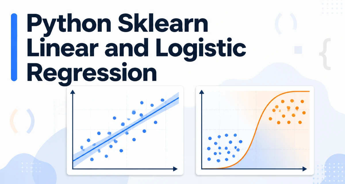
When you need to implement python sklearn linear and logistic regression, the library provides two straightforward estimators: LinearRegression and LogisticRegression. Both follow the same fit/predict pattern, but they solve different problems: regression predicts a continuous value, while classification predicts a discrete class. This article walks through the core usage, the parameters that matter, and the practical decisions you need to make.
Setting Up the Environment
Install scikit-learn if you haven't already:
pip install scikit-learn
Then import the classes you need. For the examples in this article, you'll also need numpy for data handling and matplotlib if you want to visualize results.
import numpy as np
from sklearn.linear_model import LinearRegression, LogisticRegression
from sklearn.model_selection import train_test_split
from sklearn.preprocessing import StandardScaler
from sklearn.metrics import mean_squared_error, r2_score, accuracy_score, confusion_matrix, roc_auc_score
Linear Regression with sklearn
LinearRegression fits a model that assumes a linear relationship between the feature matrix X and the target vector y. The model learns coefficients w and an intercept b to minimize the residual sum of squares.
Here's a minimal example using synthetic data:
# Generate synthetic data
np.random.seed(42)
X = np.random.rand(100, 1) * 10
y = 2.5 * X.squeeze() + np.random.randn(100) * 2

# Split into train and test sets
X_train, X_test, y_train, y_test = train_test_split(X, y, test_size=0.2, random_state=42)

# Create and train the model
model = LinearRegression()
model.fit(X_train, y_train)

# Predict and evaluate
predictions = model.predict(X_test)
print(f"Coefficient: {model.coef_[0]:.2f}")
print(f"Intercept: {model.intercept_:.2f}")
print(f"R²: {r2_score(y_test, predictions):.2f}")
print(f"MSE: {mean_squared_error(y_test, predictions):.2f}")
The fit method computes the coefficients using the ordinary least squares solution. The coef_ attribute holds the weights for each feature, and intercept_ holds the bias term. The predict method returns continuous values.
Key Parameters
fit_intercept: Whether to calculate the intercept. Set toFalseif you know the data is centered at zero.positive: IfTrue, forces coefficients to be non-negative. Useful when domain knowledge requires non-negative weights.
Logistic Regression with sklearn
LogisticRegression is used for classification, despite its name. It models the probability that an instance belongs to a particular class using the logistic (sigmoid) function. The default solver works well for most datasets, but you may need to adjust parameters for large or high-dimensional data.
# Generate binary classification data
np.random.seed(42)
X = np.random.randn(200, 2)
y = (X[:, 0] + X[:, 1] > 0).astype(int)

# Split
X_train, X_test, y_train, y_test = train_test_split(X, y, test_size=0.2, random_state=42)

# Train
clf = LogisticRegression()
clf.fit(X_train, y_train)

# Predict and evaluate
preds = clf.predict(X_test)
probs = clf.predict_proba(X_test)[:, 1]  # probability for class 1
print(f"Accuracy: {accuracy_score(y_test, preds):.2f}")
print(f"AUC: {roc_auc_score(y_test, probs):.2f}")
predict returns the class label (0 or 1 by default), while predict_proba returns the probability estimates for each class. The decision threshold is 0.5 by default, but you can adjust it manually if you need to trade off precision and recall.
Key Parameters
penalty: Regularization type ('l1','l2','elasticnet', or'none'). Default is'l2'.C: Inverse of regularization strength. Smaller values mean stronger regularization.solver: Algorithm to use ('lbfgs','liblinear','newton-cg', etc.). The default'lbfgs'is a good starting point.
Key Differences Between Linear and Logistic Regression
| Aspect | Linear Regression | Logistic Regression |
|---|---|---|
| Output | Continuous value | Probability or class label |
| Loss function | Mean squared error | Log loss (cross-entropy) |
| Model form | Linear combination of features | Sigmoid applied to linear combination |
| Evaluation metrics | R², MSE, RMSE | Accuracy, precision, recall, AUC |
| Assumptions | Linearity, homoscedasticity | No strict linearity, but decision boundary is linear |
These differences dictate how you preprocess data and interpret results. For regression, you care about residual distribution; for classification, you care about class separation and probability calibration.
Feature Scaling and Regularization
Both models can benefit from feature scaling, but it's critical for logistic regression with regularization. When features have different scales, the regularization term penalizes coefficients unevenly, leading to biased model selection. Scaling ensures each feature contributes equally to the penalty.
Use StandardScaler to standardize features before fitting:
scaler = StandardScaler()
X_train_scaled = scaler.fit_transform(X_train)
X_test_scaled = scaler.transform(X_test)

clf = LogisticRegression(C=1.0)
clf.fit(X_train_scaled, y_train)
For linear regression, scaling is less critical because the closed-form solution is scale-invariant, but it helps when you use gradient-based solvers or when you want to interpret coefficients as standardized weights.
Regularization prevents overfitting. In LogisticRegression, the C parameter controls the strength: lower C increases regularization. For LinearRegression, you would use Ridge or Lasso for L2 or L1 regularization, but LinearRegression itself has no regularization.
Evaluating Model Performance
For regression, common metrics are R² (coefficient of determination) and mean squared error (MSE). R² indicates how much variance in the target is explained by the model. MSE gives the average squared error in the same units as the target.
For classification, accuracy is simple but can be misleading with imbalanced classes. Use confusion matrices and ROC-AUC to get a fuller picture:
from sklearn.metrics import confusion_matrix, classification_report

cm = confusion_matrix(y_test, preds)
print(cm)
print(classification_report(y_test, preds))
The confusion matrix shows true positives, false positives, true negatives, and false negatives. The classification report includes precision, recall, and F1-score per class.
Handling Multiclass Classification
LogisticRegression supports multiclass classification out of the box. By default, it uses a one-vs-rest (OvR) strategy, but you can switch to multinomial (softmax) by setting multi_class='multinomial' and choosing a compatible solver like 'lbfgs'.
# Three-class example
X = np.random.randn(150, 2)
y = np.random.choice([0, 1, 2], size=150)

clf = LogisticRegression(multi_class='multinomial', solver='lbfgs')
clf.fit(X_train, y_train)
Multinomial regression treats all classes simultaneously, which often gives better probability estimates than OvR when classes are mutually exclusive.
Common Pitfalls and Practical Considerations
One frequent mistake is scaling the entire dataset before splitting. This causes data leakage because the scaler sees the test set statistics. Always fit the scaler on the training set only, then transform the test set.
Another issue is ignoring class imbalance. If one class is rare, accuracy can be high while the model fails to predict the minority class. Use class_weight='balanced' in LogisticRegression to automatically adjust weights inversely proportional to class frequencies.
Solver choice matters for large datasets. 'lbfgs' works well for small to medium data, but 'saga' is better for large sparse datasets and supports L1 regularization. For linear regression, the default solver uses the singular value decomposition, which is stable but can be slow for very high-dimensional data; consider Ridge with solver='sparse_cg' if memory is a concern.
Finally, interpret coefficients carefully. In logistic regression, a coefficient represents the log-odds change for a one-unit increase in the feature, holding others constant. In linear regression, it's the change in the target for a one-unit increase. Always consider the feature scale when comparing coefficients across features.