Python Sklearn PCA: Dimensionality Reduction Explained

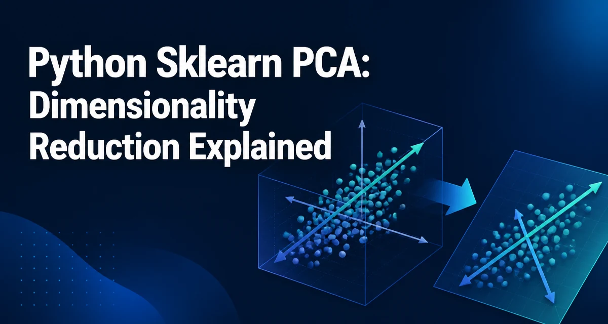
When you need to reduce the dimensionality of a dataset, python sklearn pca dimensionality reduction is a standard technique. PCA (Principal Component Analysis) projects data onto a new set of orthogonal axes that capture the maximum variance. This is useful for visualization, noise reduction, and speeding up downstream algorithms.

What PCA Does and When to Use It

PCA finds linear combinations of the original features that explain the most variance. The first principal component points in the direction of greatest variance, the second is orthogonal to the first and captures the next largest variance, and so on. By keeping only the first few components, you compress the data while retaining the structure that matters most.

Use PCA when:

• You have many correlated features and want to remove redundancy.
• You need to visualize high-dimensional data in 2D or 3D.
• You want to reduce training time for models that scale poorly with feature count.
• You suspect the intrinsic dimensionality is much lower than the number of features.

PCA is a linear method, so it won't capture nonlinear relationships. For that, consider techniques like t-SNE or UMAP, but PCA remains a fast and interpretable first step.

Preparing Data for PCA

PCA is sensitive to the scale of the features. If one feature has a range of 0–1000 and another is 0–1, the first will dominate the variance even if it's not more informative. Standardize the data so each feature has zero mean and unit variance before applying PCA.

from sklearn.preprocessing import StandardScaler
from sklearn.decomposition import PCA

scaler = StandardScaler()
X_scaled = scaler.fit_transform(X)

StandardScaler subtracts the mean and divides by the standard deviation for each column. This ensures all features contribute equally to the variance calculation.

Applying PCA with sklearn

The PCA class in sklearn is straightforward. You fit it on the scaled data and then transform the original data into the reduced space.

pca = PCA(n_components=2)
X_pca = pca.fit_transform(X_scaled)

n_components sets the number of principal components to keep. After fitting, you can inspect how much variance each component explains.

print(pca.explained_variance_ratio_)

This array shows the proportion of total variance captured by each component. The sum of these values tells you how much variance you retained overall.

Choosing the Number of Components

There's no universal answer for n_components. A common approach is to plot the cumulative explained variance and look for an elbow where adding more components yields diminishing returns.

import matplotlib.pyplot as plt

pca_full = PCA().fit(X_scaled)
cumulative_variance = pca_full.explained_variance_ratio_.cumsum()

plt.plot(range(1, len(cumulative_variance) + 1), cumulative_variance)
plt.xlabel('Number of Components')
plt.ylabel('Cumulative Explained Variance')
plt.show()

Alternatively, you can set n_components to a float between 0 and 1 to keep the minimum number of components that explain at least that fraction of variance. For example, PCA(n_components=0.95) retains enough components to explain 95% of the variance.

Interpreting the Results

The transformed data X_pca has rows corresponding to original samples and columns to the selected principal components. These components are linear combinations of the original features. The components_ attribute of the fitted PCA object gives the loadings, which show how much each original feature contributes to each component.

loadings = pca.components_

For the first component, a large positive loading on a feature means that feature strongly influences that component. This can help you understand what the component represents, though interpretation becomes harder with many features.

Practical Considerations: Scaling, Variance, and Performance

Scaling is not optional for PCA. Without standardization, the method becomes a function of the units you chose, not the underlying structure. Always apply StandardScaler or a similar transformation before PCA.

PCA is computationally efficient for moderate-sized datasets. The cost is dominated by the singular value decomposition (SVD) used internally. For very large datasets, you can use PCA with svd_solver='randomized' to approximate the components faster, at a slight cost in accuracy. This is useful when you have many features or samples.

pca = PCA(n_components=10, svd_solver='randomized')

The randomized solver is especially effective when you only need a small number of components relative to the feature count.

Common Pitfalls and Limitations

One common mistake is applying PCA to data that hasn't been scaled. Another is using PCA on categorical features, which is inappropriate because PCA assumes numeric, continuous variables. Also, PCA is a linear projection; if the data lies on a nonlinear manifold, PCA may not capture the structure.

When you use PCA for visualization, the axes are not directly interpretable as original features. You need to be careful when drawing conclusions from the positions of points in the reduced space.

Finally, PCA is unsupervised. It doesn't use the target variable, so it may discard information that is useful for classification or regression. If you want to reduce dimensionality while preserving class separability, consider supervised methods like Linear Discriminant Analysis.

Example: PCA for Visualization

A common use case is visualizing high-dimensional data in two dimensions. After scaling and applying PCA, you can plot the transformed points and color them by a target variable if available.

import matplotlib.pyplot as plt

pca = PCA(n_components=2)
X_pca = pca.fit_transform(X_scaled)

plt.scatter(X_pca[:, 0], X_pca[:, 1], c=y, cmap='viridis')
plt.xlabel('First Principal Component')
plt.ylabel('Second Principal Component')
plt.colorbar()
plt.show()

This gives a quick view of how well-separated the classes are in the reduced space. It's often the first step in exploratory data analysis.

When PCA Is Not the Right Tool

If you need to preserve the original feature names for interpretation, PCA replaces them with abstract components. In that case, feature selection methods like SelectKBest might be more appropriate. Also, if your data has missing values, you'll need to handle them before PCA, as sklearn's PCA does not accept NaN values.

For high-dimensional sparse data, such as text represented as TF-IDF vectors, PCA is not efficient because it densifies the data. Truncated SVD (via sklearn.decomposition.TruncatedSVD) works better for sparse matrices.