Comparing Python sklearn SVM, KNN, and Naive Bayes
python sklearn svm knn and naive bayes: Implement SVM, KNN, and naive Bayes classifiers in scikit-learn, compare their tradeoffs, and choose the right algorithm for yo...
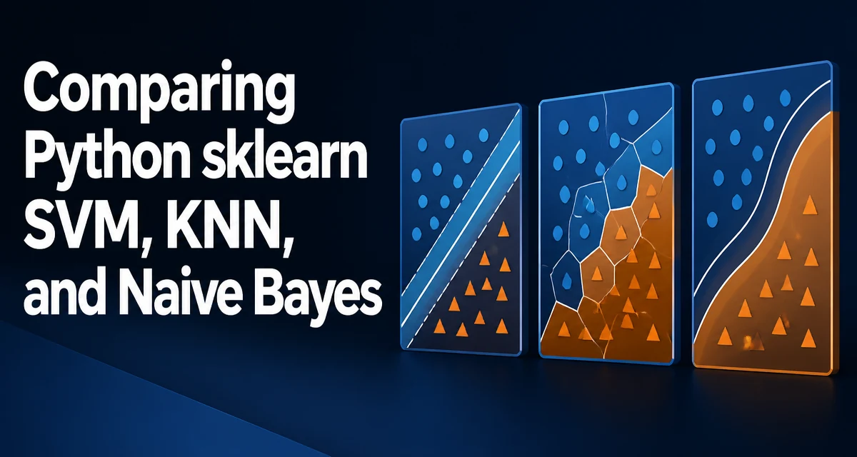
Choosing a classification algorithm in scikit-learn often comes down to three familiar names: support vector machines (SVM), k-nearest neighbors (KNN), and naive Bayes. The right choice depends on your dataset size, feature dimensionality, and how much you care about prediction speed. This article shows how to implement python sklearn svm knn and naive bayes classifiers and explains the tradeoffs that matter in practice.
How Each Classifier Makes Decisions
SVM finds a hyperplane that separates classes with the maximum margin. With a kernel, it can project data into a higher-dimensional space to handle non-linear boundaries. The decision function depends only on support vectors, the training points closest to the margin.
KNN stores the entire training set and classifies a new point by looking at the majority class among its k nearest neighbors. The decision boundary is local and non-parametric, shaped entirely by the training data distribution.
Naive Bayes applies Bayes' theorem with a strong independence assumption between features. For each class, it estimates the probability of a feature value given that class, then combines these probabilities to predict the most likely label. The Gaussian variant assumes each feature follows a normal distribution within a class.
These differences drive everything from training cost to prediction speed and sensitivity to feature scaling.
Implementing SVM with scikit-learn
The SVC class in scikit-learn provides a flexible SVM implementation. For a typical classification task, you instantiate the model, fit it on scaled features, and call predict.
from sklearn.svm import SVC
from sklearn.datasets import load_iris
from sklearn.model_selection import train_test_split
from sklearn.preprocessing import StandardScaler

X, y = load_iris(return_X_y=True)
X_train, X_test, y_train, y_test = train_test_split(X, y, test_size=0.3, random_state=42)

scaler = StandardScaler()
X_train_scaled = scaler.fit_transform(X_train)
X_test_scaled = scaler.transform(X_test)

svm_model = SVC(kernel='rbf', C=1.0, gamma='scale')
svm_model.fit(X_train_scaled, y_train)
accuracy = svm_model.score(X_test_scaled, y_test)
print(f'SVM accuracy: {accuracy:.3f}')
Feature scaling is critical for SVM because the margin is computed from distances. Without scaling, features with larger ranges dominate the distance calculation. The kernel parameter controls the decision boundary shape; rbf is a common default for non-linear data. C trades off misclassification tolerance against margin width, and gamma defines how far a single training point influences the model.
Implementing K-Nearest Neighbors with scikit-learn
KNeighborsClassifier is straightforward: you set the number of neighbors k, fit the model, and predict. The training step is essentially storing the data, so it is fast, but prediction requires scanning the training set for each query.
from sklearn.neighbors import KNeighborsClassifier

knn_model = KNeighborsClassifier(n_neighbors=5)
knn_model.fit(X_train_scaled, y_train)
accuracy = knn_model.score(X_test_scaled, y_test)
print(f'KNN accuracy: {accuracy:.3f}')
KNN also depends on distance, so scaling is equally important. The n_neighbors value controls the smoothness of the decision boundary. Small values fit noise, while large values smooth out class distinctions. KNN has no explicit training phase, but prediction time grows linearly with the number of training samples, which becomes a problem for large datasets.
Implementing Naive Bayes with scikit-learn
For continuous features, GaussianNB is the typical choice. It estimates the mean and variance of each feature per class during training. Prediction is a simple probability calculation, making it extremely fast.
from sklearn.naive_bayes import GaussianNB

nb_model = GaussianNB()
nb_model.fit(X_train, y_train)
accuracy = nb_model.score(X_test, y_test)
print(f'Naive Bayes accuracy: {accuracy:.3f}')
Naive Bayes does not require feature scaling because it models each feature independently. This is a practical advantage when you have mixed-scale features or when scaling is inconvenient. However, the independence assumption can hurt accuracy if features are strongly correlated. The model also tends to give well-calibrated probabilities when the assumption holds, but it can be overconfident otherwise.
Comparing the Three Classifiers
The following table summarizes the key differences you should consider when selecting among these algorithms.
| Criterion | SVM | KNN | Naive Bayes |
|---|---|---|---|
| Training time | Moderate for small/medium data | Trivial (stores data) | Very fast |
| Prediction time | Fast (depends on support vectors) | Slow (scans all training data) | Very fast |
| Interpretability | Low (kernel space is opaque) | Moderate (local neighbors) | High (per-feature probabilities) |
| Feature scaling | Required | Required | Not required |
| Handles high dimensions | Good with kernels, but risks overfitting | Poor (distance concentration) | Excellent (works well with many features) |
| Non-linear boundaries | Yes, with kernel | Yes, naturally | Only with feature engineering |
These differences are not just theoretical. They directly affect how you preprocess data, how long training takes, and how quickly you can serve predictions in production.
Choosing the Right Classifier for Your Data
The best algorithm depends on the structure of your problem. Use SVM when you have a small to medium dataset with a clear margin between classes and you can afford to tune the kernel and regularization parameters. It is especially effective when the number of features is moderate and you need a robust decision boundary.
Choose KNN when you have a small dataset, the decision boundary is highly irregular, and you need a model that adapts to local structure without training. It is also a reasonable baseline because it has no training phase, but you must be prepared for slow predictions if the dataset grows.
Prefer Naive Bayes when you have high-dimensional data, such as text or sensor streams, where the independence assumption is acceptable or where training speed and memory are more important than peak accuracy. It is also a strong choice when you need a fast, interpretable model that can be retrained frequently.
If your data has strongly correlated features, consider whether Naive Bayes's independence assumption will cause systematic errors. In that case, SVM or KNN may capture the interaction better, even if they require more careful preprocessing.
Performance and Scalability Considerations
SVM training involves solving a quadratic optimization problem. For a few thousand samples, this is manageable, but it becomes slow as the dataset grows. The number of support vectors also affects prediction time, though usually far less than KNN's full scan.
KNN has no training cost, but every prediction requires computing distances to all training points. With a million samples, that is a million distance calculations per prediction. Techniques like KD-trees or ball trees can speed up exact neighbor search, but they degrade in high dimensions. In practice, KNN is rarely the right choice for large production datasets.
Naive Bayes is the most scalable of the three. Training is a single pass over the data to compute per-class statistics, and prediction is a few multiplications per feature. This makes it ideal for online learning or batch processing on massive datasets. The tradeoff is that the independence assumption can limit accuracy, so you must decide whether that cost is acceptable.
Memory usage follows a similar pattern. KNN stores the entire training set, SVM stores support vectors, and Naive Bayes stores only the class priors and feature statistics. If you are deploying to a constrained environment, Naive Bayes is the clear winner.
Common Pitfalls and How to Avoid Them
One frequent mistake is forgetting to scale features for SVM and KNN. If you fit a scaler on the training set, you must apply the same transformation to the test set and to any new data in production. Forgetting to reuse the scaler leads to silently degraded predictions.
Another pitfall is choosing an inappropriate k for KNN. A very small k like 1 produces a jagged boundary that overfits, while a very large k oversmooths and may miss local structure. Use cross-validation to select k rather than relying on a default.
For SVM, the default gamma='scale' works reasonably, but you should tune both C and gamma together. A high gamma can cause overfitting, and a low C can underfit. Grid search with cross-validation is the standard way to find good values.
Naive Bayes often fails when features are highly correlated. If you know that two features are redundant, consider removing one or using a more flexible model. Also, GaussianNB assumes normally distributed features; if your data is heavily skewed, a log transform can improve the fit.
Finally, be careful when comparing accuracy across these models without considering the cost of misclassification. SVM and KNN can produce more balanced errors, while Naive Bayes may be overconfident in one class. Always evaluate precision, recall, and the confusion matrix in addition to overall accuracy.