Python Transformers Embeddings and Feature Extraction

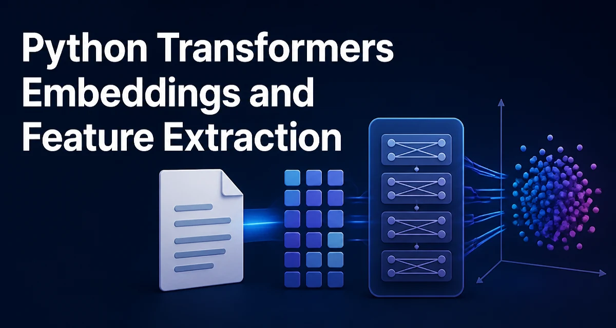
python transformers embeddings and feature extraction requires a clear understanding of the core syntax, runtime behavior, and practical implementation patterns demonstrated in the examples below.

When working with Python Transformers, extracting embeddings and feature vectors from text is a common task for downstream machine learning models. The transformers library provides pretrained models that produce contextual representations, but the raw output requires careful handling before it becomes a usable embedding. This article explains the full pipeline: loading a model, tokenizing input, extracting hidden states, choosing a pooling strategy, and normalizing the result for similarity or classification tasks.

What You Get From a Transformer Model

A transformer model like BERT or RoBERTa does not directly output a single vector for a sentence. Instead, it returns a last_hidden_state tensor with shape (batch_size, sequence_length, hidden_size). Each token in the input sequence gets a contextualized vector. For example, a sentence with 10 tokens produces 10 vectors, each of dimension 768 for base-sized models. The final hidden state is the input to the pooling step.

Some models also provide a pooler_output, which is a single vector derived from the first token's hidden state after a linear layer and activation. This is often used for classification heads, but it is not always the best choice for semantic similarity. Understanding what the model returns is the first step in building a reliable feature extraction pipeline.

Loading a Pretrained Model and Tokenizer

The standard way to load a model is through the AutoModel and AutoTokenizer classes. These automatically select the correct architecture based on the model identifier. For example, "bert-base-uncased" loads a BERT model with a vocabulary of about 30,000 tokens.

from transformers import AutoTokenizer, AutoModel

model_name = "bert-base-uncased"
tokenizer = AutoTokenizer.from_pretrained(model_name)
model = AutoModel.from_pretrained(model_name)

The model is loaded in evaluation mode by default when using from_pretrained, but it is still good practice to call model.eval() if you plan to reuse it for inference. If you are using a GPU, move the model with model.to("cuda"). The tokenizer remains on the CPU and handles text preprocessing.

Tokenizing Input and Preparing Batches

The tokenizer converts raw text into input IDs, attention masks, and token type IDs (for models that use them). The __call__ method handles padding and truncation automatically when you pass the appropriate arguments. For feature extraction, you typically want to pad to the longest sequence in the batch and truncate to the model's maximum length.

texts = ["The quick brown fox jumps over the lazy dog.", "Transformers encode context efficiently."]

inputs = tokenizer(texts, padding=True, truncation=True, return_tensors="pt")

The return_tensors="pt" key returns PyTorch tensors. If you are using TensorFlow, use "tf" instead. The resulting inputs dictionary contains input_ids and attention_mask. The attention mask tells the model which tokens are real and which are padding, so it is essential to pass it during the forward pass.

Extracting Embeddings From Hidden States

With the tokenized inputs, you can run the model and access the hidden states. The model returns a BaseModelOutput object, and the last_hidden_state attribute contains the token-level vectors.

with torch.no_grad():
    outputs = model(**inputs)
    last_hidden = outputs.last_hidden_state

The torch.no_grad() context disables gradient computation, which reduces memory usage and speeds up inference. If you are not fine-tuning the model, this is the correct way to run forward passes. The last_hidden tensor now holds the contextualized token vectors for every token in the batch.

Choosing a Pooling Strategy: CLS Token vs Mean Pooling

The token-level vectors must be reduced to a single vector per sequence. Two common strategies are using the CLS token's hidden state and mean pooling over all token vectors. The CLS token is the first token in BERT-style models, and its final hidden state is designed to aggregate information for classification tasks. However, for semantic similarity, mean pooling often produces better results because it averages information from all tokens rather than relying on a single position.

Mean pooling should respect the attention mask to exclude padding tokens. A naive average over all tokens would include zeros from padded positions, diluting the representation. The correct implementation multiplies each token vector by the attention mask and divides by the sum of the mask values.

import torch

# inputs['attention_mask'] has shape (batch_size, sequence_length)
mask = inputs['attention_mask'].unsqueeze(-1).float()
summed = (last_hidden * mask).sum(dim=1)
counts = mask.sum(dim=1).clamp(min=1e-9)
mean_pooled = summed / counts

The clamp prevents division by zero for sequences that are entirely padding, which should not happen in practice. The resulting mean_pooled tensor has shape (batch_size, hidden_size).

Normalizing Embeddings for Similarity Search

After pooling, the embeddings often need to be normalized to unit length before computing cosine similarity. Cosine similarity is equivalent to the dot product of L2-normalized vectors. Many downstream tasks, such as retrieval or clustering, assume normalized embeddings. Normalization also makes the embeddings more stable when used with approximate nearest neighbor libraries.

normalized = torch.nn.functional.normalize(mean_pooled, p=2, dim=1)

Once normalized, the dot product between two vectors gives their cosine similarity. This is the standard approach for sentence embeddings. If you plan to use the embeddings as features for a linear classifier, normalization is not always required, but it rarely hurts and often helps convergence.

Batch Processing and GPU Considerations

Extracting embeddings for many texts requires batching to avoid excessive memory usage and to utilize GPU parallelism. The tokenizer can handle a list of strings in one call, but for very large datasets you should process in chunks. A common pattern is to iterate over the dataset in batches of 32 or 64, depending on the model size and GPU memory.

def extract_embeddings(texts, batch_size=32):
    embeddings = []
    for i in range(0, len(texts), batch_size):
        batch = texts[i:i+batch_size]
        inputs = tokenizer(batch, padding=True, truncation=True, return_tensors="pt")
        inputs = {k: v.to(model.device) for k, v in inputs.items()}
        with torch.no_grad():
            outputs = model(**inputs)
            last_hidden = outputs.last_hidden_state
        mask = inputs['attention_mask'].unsqueeze(-1).float()
        summed = (last_hidden * mask).sum(dim=1)
        counts = mask.sum(dim=1).clamp(min=1e-9)
        mean_pooled = summed / counts
        normalized = torch.nn.functional.normalize(mean_pooled, p=2, dim=1)
        embeddings.append(normalized.cpu())
    return torch.cat(embeddings, dim=0)

Moving inputs to the model's device is important when using a GPU. The output is moved back to CPU to avoid accumulating GPU memory. Padding to the longest sequence in each batch means that batch size and sequence length trade off against memory. Shorter batches with longer sequences may be necessary for memory-constrained environments.

Using the Feature Extraction Pipeline for Quick Prototyping

The transformers library includes a high-level pipeline that abstracts away the tokenization and pooling steps. For feature extraction, you can create a pipeline with the task "feature-extraction" and specify a model.

from transformers import pipeline

feature_extractor = pipeline("feature-extraction", model="bert-base-uncased")
result = feature_extractor("The quick brown fox jumps over the lazy dog.")

The output is a list of token-level vectors, not a single pooled vector. The pipeline does not apply pooling by default, so you still need to implement mean pooling or CLS extraction yourself. The pipeline is convenient for quick experiments, but for production batch processing, the manual approach gives you more control over padding, device placement, and pooling.

One limitation of the pipeline is that it returns Python lists, which can be slow for large datasets. For performance-critical applications, using the underlying model directly is preferable. The pipeline also does not normalize the output, so you must apply normalization if you need unit-length embeddings.

When choosing between the pipeline and the manual method, consider whether you need to customize the pooling strategy, handle large batches efficiently, or integrate with a larger PyTorch or TensorFlow workflow. For a one-off script, the pipeline reduces boilerplate. For a service that processes millions of texts, the manual approach is more maintainable and easier to optimize.