PyTorch Training and Validation Loops in Python
python pytorch training and validation loops: Learn how to structure PyTorch training and validation loops, handle device placement, manage gradients, and avoid common...
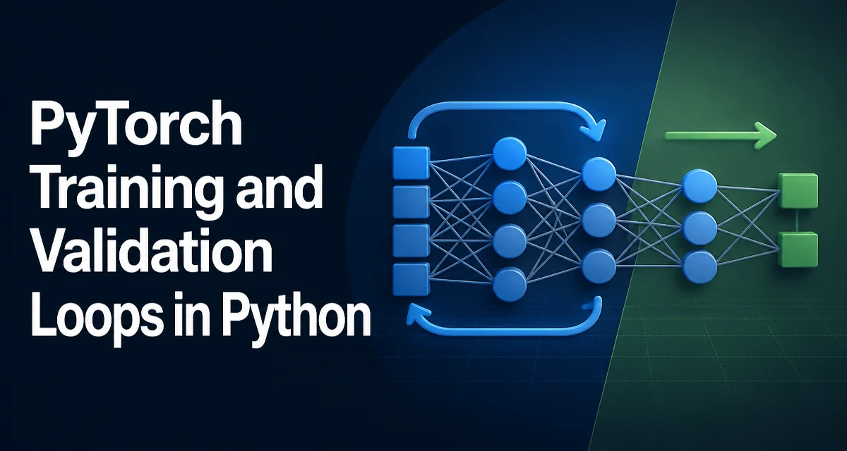
A PyTorch training loop is the code that repeatedly feeds batches of data through a model, computes a loss, and updates the model's parameters. A validation loop runs the same model on held-out data without updating parameters. Together they form the core of every supervised deep learning workflow in Python. This article explains how to structure python pytorch training and validation loops correctly, what each function call does, and where common failures occur.
The Structure of a PyTorch Training Loop
A training loop in PyTorch follows a consistent pattern: forward pass, loss computation, backward pass, and optimizer step. The loop iterates over batches from a DataLoader, moves data to the appropriate device, and updates model parameters.
for epoch in range(num_epochs):
    model.train()
    for batch in train_loader:
        inputs, targets = batch
        inputs = inputs.to(device)
        targets = targets.to(device)

        optimizer.zero_grad()
        outputs = model(inputs)
        loss = criterion(outputs, targets)
        loss.backward()
        optimizer.step()
The model.train() call sets the model to training mode, which enables dropout and batch normalization behavior that depends on training state. The optimizer.zero_grad() call clears gradients from the previous iteration; without it, gradients accumulate across batches and the parameter update becomes incorrect.
The Validation Loop and Why It Differs
Validation loops evaluate the model on held-out data without updating parameters. The critical difference is the torch.no_grad() context, which disables gradient tracking and reduces memory usage.
model.eval()
total_loss = 0.0
correct = 0
total = 0

with torch.no_grad():
    for batch in val_loader:
        inputs, targets = batch
        inputs = inputs.to(device)
        targets = targets.to(device)

        outputs = model(inputs)
        loss = criterion(outputs, targets)
        total_loss += loss.item() * inputs.size(0)

        _, predicted = torch.max(outputs, 1)
        correct += (predicted == targets).sum().item()
        total += targets.size(0)

avg_val_loss = total_loss / total
val_accuracy = correct / total
The model.eval() call switches batch normalization to use running statistics instead of batch statistics and disables dropout. Failing to call model.eval() before validation produces misleading metrics because the model behaves differently during inference than during training.
Device Placement: Moving Data and Model to GPU
PyTorch requires explicit device management. The model and every tensor must reside on the same device for operations to succeed.
device = torch.device("cuda" if torch.cuda.is_available() else "cpu")
model = model.to(device)
Moving data to the device inside the loop is the most common pattern, but the DataLoader can handle it more efficiently with pin_memory=True when using CUDA. The to(device) call on each batch remains necessary because the DataLoader yields CPU tensors by default.
Loss Computation and Backpropagation Details
The loss function receives model outputs and targets. For classification, nn.CrossEntropyLoss expects raw logits, not softmax probabilities. The backward pass computes gradients for every parameter that requires gradients.
criterion = nn.CrossEntropyLoss()
optimizer = optim.Adam(model.parameters(), lr=1e-3)
The order matters: zero_grad() must come before backward(), and step() must come after. Calling backward() without zeroing gradients accumulates them, which changes the effective batch size and can destabilize training.
Gradient Accumulation as a Deliberate Technique
Gradient accumulation is sometimes intentional, particularly when memory constraints prevent large batch sizes. The pattern involves skipping the optimizer step for several iterations.
accumulation_steps = 4
optimizer.zero_grad()

for i, batch in enumerate(train_loader):
    inputs, targets = batch
    inputs = inputs.to(device)
    targets = targets.to(device)

    outputs = model(inputs)
    loss = criterion(outputs, targets) / accumulation_steps
    loss.backward()

    if (i + 1) % accumulation_steps == 0:
        optimizer.step()
        optimizer.zero_grad()
Dividing the loss by the accumulation steps normalizes the gradient magnitude so the effective learning rate matches a full batch. This technique trades memory for training time and is most useful when the model or input size makes a single large batch infeasible.
Common Pitfalls in Training and Validation Loops
Several mistakes appear repeatedly in PyTorch training code. Calling model.eval() without wrapping validation in torch.no_grad() wastes memory but produces correct results. Calling model.train() after validation is essential before the next training epoch; forgetting it leaves the model in eval mode, which disables dropout and changes batch normalization behavior during training.
Another common issue is computing accuracy incorrectly. The torch.max(outputs, 1) call returns both values and indices; taking [1] gives the predicted class. Comparing predicted classes to targets requires both tensors to be on the same device and have compatible shapes.
Performance Considerations for Training Loops
The DataLoader's num_workers parameter controls how many subprocesses load and preprocess data. Setting it to zero runs data loading in the main process, which often becomes a bottleneck for GPU training. Values between 2 and 8 are typical, but the optimal setting depends on the dataset size and preprocessing cost.
pin_memory=True in the DataLoader enables faster host-to-device transfers when CUDA is available. The effect is most visible with large batches or high-resolution inputs. On CPU-only training, pin_memory has no effect.
The torch.no_grad() context in validation avoids building the autograd graph, which reduces memory consumption and speeds up inference. For large validation sets, this difference is substantial.
Tracking Metrics Across Epochs
Accumulating loss and accuracy across batches requires care with the loss value. The loss.item() call detaches the scalar from the autograd graph, allowing it to be stored in a Python number. Summing loss.item() across batches and dividing by the total number of samples gives the average loss per sample, which is comparable across runs with different batch sizes.
epoch_loss = 0.0
num_samples = 0

for batch in train_loader:
    inputs, targets = batch
    inputs = inputs.to(device)
    targets = targets.to(device)

    optimizer.zero_grad()
    outputs = model(inputs)
    loss = criterion(outputs, targets)
    loss.backward()
    optimizer.step()

    epoch_loss += loss.item() * inputs.size(0)
    num_samples += inputs.size(0)

avg_epoch_loss = epoch_loss / num_samples
Weighting the loss by batch size prevents batches of different sizes from contributing equally to the epoch average. This matters when the final batch is smaller than the batch size, which is common with most datasets.